Descriptive Statistics

Statistics is a branch of mathematics that includes collection, organization, and interpretation of data. After collecting the data, it is the utmost priority to read and understand the data by using statistical technique before using an algorithm and making predictions.

Descriptive statistics and inferential statistic are two types of statistics. Descriptive statistics is used to obtain summary and concise view of the data whereas inferential statistics is used to make inferences about the population from the random sample of the data from a population. This blog focusses only on descriptive statistics. Descriptive statistics can be further divided into:

1. Measures of central tendency
2. Measures of variability
3. Measures of relationship between variables

Data

Following data is used for explaining the computation of measures of central tendency and measures of variability

Salary of 5 employees: 7K, 6.6K, 7.5K, 8.9K, 7.5K.

1. Measures of central tendency

A measure of central tendency is a summary of the data that represents a whole set of data with a unique value or a point that represents the center or middle of its distribution. There are three measures of central tendency namely mean, median and mode.

Mean

Mean is the average of all the numbers in a dataset or in other word, it is sum of all the numbers in a dataset divided by numbers of data in a dataset. Following is the formula for the population and sample mean.

Where, X is the population data and x is the sample data. N and n are the total number of data in population and sample data respectively. Mean salary can be computed as follows

Advantage of the mean

1. The mean can be employed for both discrete and continuous numerical data.

Limitations of the mean

1. The mean cannot be used for categorical data.
2. The mean is highly influenced by outliers and skewed distributions.

Median

It is a middle value in an ordered dataset where data is arranged in ascending or descending order.

To compute the median, arrange the data in ascending order which is 6.6K, 7K, 7.5K, 7.5K, 8.9K. Number of data is odd. Hence, median salary is (5+1)/2 = 3rd item in the list which is 7.5K.

Data having even number of data points : 7K, 6.6K, 7.5K, 8.9K, 7.5K and 7K.

To compute the median, arrange the data in ascending order which is 6.6K, 7K, 7K, 7.5K, 7.5K, 8.9K. Median salary is the average of 6/2 = 3rd item and (6/2+1) = 4th item in the list. Here, the 3rd and 4th numbers is 7K and 7.5K. Median salary is the average of these two numbers which is equal to (7K+7.5K)/2 = 7.25K.

Advantages of median

1. The median is less influenced by outliers and skewed data compared to that of the mean due to which it is normally the chosen measure of central tendency when the distribution is asymmetrical.
2. The median can be used for ordinal dataset.

Limitation of the median

1. The median cannot be used for nominal data as it cannot be ordered.

Mode

It is the value of a dataset having the highest frequency. If there are no items having frequency greater than 1 then there is no mode. If there are several items having frequency greater than one, there is more than one mode, also known as bimodal or multimodal.

In the data set 7K, 6.6K, 7.5K, 8.9K,7.5K, value 7.5K appears for 2 times which is the highest frequency. So, mode salary is 7.5K

Advantage of median

1. The mode can be used for numerical, ordinal and nominal data.

Influence of outliers

Outliers are an extreme value that is distinctly unusual from the rest of the data in a dataset. It is essential to identify outliers present in a distribution as it can change the results of the data analysis significantly. The mean is more sensitive to the presence of outliers than the median and mode. If the outlier is confirmed as a valid extreme value, it should not be removed from the dataset and vice versa

Example 1: Salary of 5 employee includes 7.5K, 6.6K, 100K, 8.9K, 7.5K. Calculate mean, median and mode?

1. Mean: Mean = (7.5K + 6.6K + 100K + 8.9K + 7.5K)/5 = 26.1K
2. Median: arrange the data in ascending order which is 6.6K, 7.5K, 7.5K, 8.9K and 100K. Median salary is (5+1)/2 = 3rd item in the list which is 7.5K.
3. Mode: Mode = number having highest frequency = 7.5K

In the dataset, one of the data 100K looks like an outlier. Due to this, only mean of the data is observed to be affected as mean of the salary is much higher than that of median and mode. Median and mode is not affected by outlier in the above example.

2. Measure of variability

A measure of variability is a measure that represents how data is spread out or scattered. Variance, standard deviation and coefficient of variation are three measures of variability.

Variance

Variance measures the dispersion of a set of data points around their mean. Variance is square of the difference between an each data point and the mean divided by number of data point. Variance measures the average degree to which each data deviates from the mean. The higher the variance, the greater the entire data range.Following is the formula for the population and sample variance.

For the given data as we computed above, mean salary is 7.5K. Variance of the dataset can be computed using below formula

Standard deviation

Standard deviation is the square root of the variance. Standard deviation has same unit as the data point so it easy to compare and understand. Following is the formula for the population and sample standard deviation.

For the given data as we computed above mean salary is 7.5K. Standard deviation of the dataset can be computed using below formula

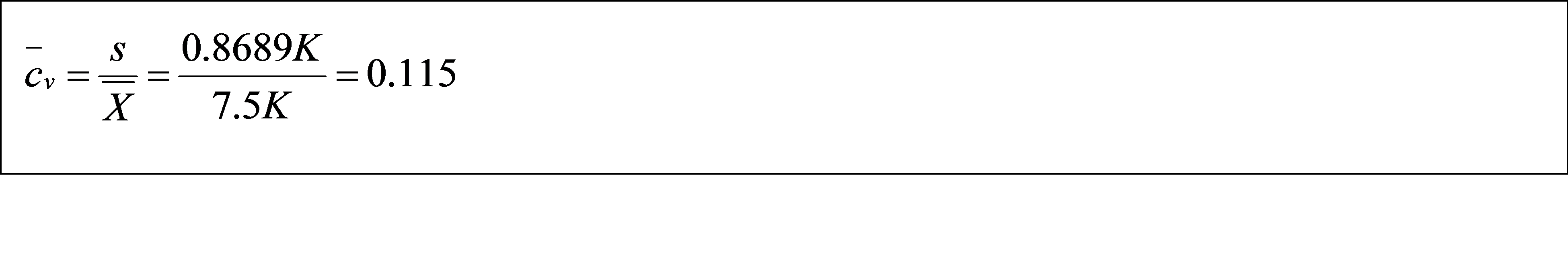
Coefficient of variation

Coefficient of variation is the relative standard deviation with respect to its mean value. Following is the formula for the population and sample coefficient of variation.

For a single dataset, standard deviation is the most common measure of variability. However, when two or more dataset are compared, comparing coefficient of variation of two or more dataset gives better insight compare to comparing standard deviation of those datasets.

For the given data as we have computed above, mean salary is 7.5K and standard deviation is 0.8689K. Coefficient of variation dataset can be found using formula

3. Measure of relationship between variables

Covariance and correlation are two measure of relationship between variables.

Covariance

Covariance is a measure indicating the degree to which two random variables changes. Its value ranges from -∞ to +∞. Following is the formula for the population and sample covariance.

Covariance gives sense of direction in the relationship between the variables. If covariance is greater than zero, the two variables move together. If it is lesser than zero, the two variables move in opposite directions. If it is equal to zero, the two variables are independent. The unit of covariance is the product of units of two variables.

Correlation

Correlation is a measure of the linear relationship between two quantitative variables. Correlation adjusts covariance so that the relationship between two variables becomes easy and intuitive to interpret. Correlation coefficient value ranges from -1 to +1. Following is the formula for the population and sample correlation coefficient.

There is a positive correlation when the values of one variable increase as the values of the other increase and vice versa. A negative correlation is when the values of one variable decrease as the values of another increase and vice versa. A correlation of one means a perfect positive correlation. A correlation of -1 means a perfect negative correlation. A correlation of 0 means that there is no relationship between the different variables. Values between -1 and 1 indicate the strength of the correlation. Some of the example of correlation are

Positive correlation

1. As more offer is given to the customers, the total sales of a company increase. Hence, offer and sales of the company are positively correlated.
2. As the salary of a person increases, the spending also increases. Hence, salary and spending are positively correlated.

Negative correlation

1. As train increases speed, the length of time required for the trip decreases. Hence, speed and time for the trip are negatively correlated.
2. As the price of the item increases, demand decreases. Hence, price and demand are negatively correlated.

Common problems in correlation

1. Correlation may not be reliable when the sample size is small.
2. If the outliers are present in the dataset, the correlation coefficient can be misleading.